What is a neural network? To get started, it’s beneficial to keep in mind that modern neural network started as an attempt to model the way that brain performs computations. We have billions of neuron cells in our brains that are connected to each other and pass information around.
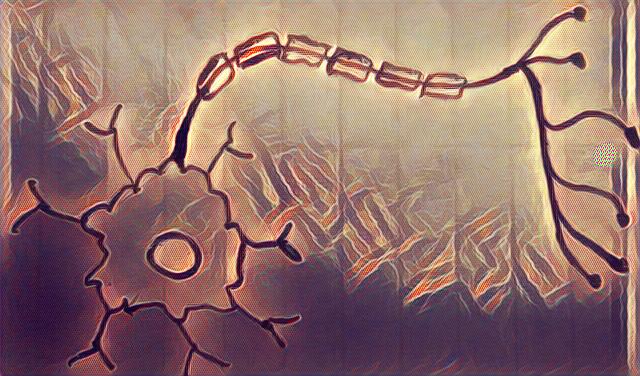
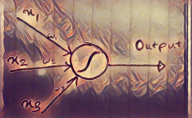
An artificial neuron is a simplified model of the neuron cell. It takes several inputs x1,x2, … and produces a linear combination of the inputs and then applies some sort of a nonlinear function to them. The parameters for the linear combination part are called weights and biases and the nonlinear function is usually a sigmoid, tanh or a simple line that is clipped at one end (rectified linear unit- ReLU). It’s important to note that such a neuron is a differentiable unit (the smoothed out version of a perceptron).
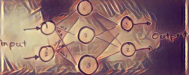
You can make a neural network by connecting several neurons with each other. A common way of doing this is by arranging them in layers so that a layer of neurons get their inputs from the previous layer and give their outputs to the next (i.e. a feedforward neural network). Feedback loops are also possible in which case the network will be called a recurrent neural network. The feedback loops will cause the neurons to fire for a limited time instead of a single firing, so in a sense they implement a type of memory.
A neural network simply recieves some inputs, performs a succession of linear combinations and nonlinearities and produces some output and the whole combination is a differentiable function. The important point is that such a network has parameters, i.e. weights and biases, that in some sense linearly scale the outputs of one layer before it goes to the next layer. You can set these parameters as whatever you want and as a result, the output of the network will change. Since the network is differentiable and nonlinearities are smooth function, small changes in parameters result in small changes in the output. It is easy to imagine that if you set parameters in some clever way, you might be able to make the network produce outputs similar to another function. In fact, it has been shown that given enough layers and neurons, a neural network can estimate any function.
So the question is how to set such clever weights and biases for different layers in the network to make it do useful things. For example, if I want my neural network to estimate a function for house prices based on size and neighborhood informations, how can I find the proper parameters? Well, the cool thing about neural networks is that they can “learn” their parameters by themselves without the need for me to set them by hand. So what does that learning mean? It means that if I have enough examples of (size, neighborhood) vs. (house price), a clever but simple optimization technique can iteratively find the best parameters for the network for this data.
How does this clever optimization work, you ask? Imagine a ball and a bowl, given the forces in the physical world, the ball will roll down the bowl and get to minimum. The same idea is used for finding minimum here. The key point to understand is that the ball rolls down in the reverse direction of the gradient at each point. So if we move in this direction we can get to the minimum of the error curve. This is how the algorithm implemented for a neural network; in the beginning, the algorithm uses some random numbers for weights and biases and then calculates an output based on the input to the network (size, neighborhood). Such an estimated output (house price) is obviously not that good since the parameters were random. Then we calculate how far this estimate is from the real value (house price) for the given input (size, neighborhood) as the error. We are interested in an error measure that is a smooth function of the network parameters for practical reasons (i.e. finding gradients). If we can reduce this error for all examples we are getting closer to good parameter values for our network. So if you imagine all error values as being plotted on a curve (the bowl), we can remember from high school calculus that the derivative (gradient) of this error is equal to the slope of the tangent line at that point. So to get to the minimum of the error curve, we simply have to move in reverse direction of gradient (we’ll get to maximum if we move in the direction of gradient). This is the clever optimization technique that we talked about earlier and is called a fancy name i.e. “stochastic gradient descent”.
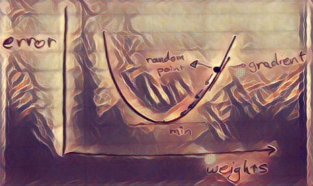
How do we move toward this minimum, you might ask? We are interested in network weights and biases that produce the minimum error. What good is the gradient of error, if we only care about finding the right parameters? Well, if you remember the chain rule for calculating derivatives, you know that you can calculate the derivative for the previous layers based on the error value at the output layer. This is called another fancy name i.e. “back-propagation”. We now have the gradient at each layer, we can just deduct a percentage (learning rate) of the derivative from each parameter according to our clever optimization technique. Each time we do this procedure, we can reduce the error and get closer to good parameters for the network.
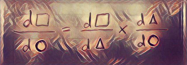
There are other techniques that are used in practice to make neural networks work on a given problem. I am not going to go into details on these, you can follow the links to learn more, but generally speaking, the workflow for solving a machine learning problem (e.g. classification) with neural networks is something like this:
1- Divide data to training and test sets for training the classifier, and assessing the performance.
2- Make a loss function, for example the log likelihood or cross entropy loss.
3- Calculate the gradients of the loss function w.r.t model parameters and backpropagate.
4- Update the parameters in batches using stochastic gradient descent or adagrad/adam/rmsprop/etc.
5- Add regularization terms to the loss function to prevent overfitting if required (a mechanism for ocam’s razor). There are L-p regularization terms which correspond to that penalize large parameters.
6- Do early stopping for improved generalization: stop training if the performance on the validation set degrades.
7- To reduce the effects of a certain division of dataset that might not be representative of all data and to reduce overfitting, we can employ a method called k-fold crossvalidation. In step 1, we further divide the training set into random segment. We reserve one segment for validation and train on the remaining segments; We repeat this process for all segments and measure performance to average all models.
This is the gist of neural networks but of course there are some details that I skipped here. The core idea is simple and elegant. You might have heard of deep learning. It is interesting to know that deep learning means just more layers between input and output. Before 2006, people thought that calculating the weights and biases would not be possible for deep network but with today’s fast GPUs and the vast amount of labeled data that we have today, it is now possible and it does wonders!